Experimental Software Fundamentals

Warning: Math Ahead

This post will serve as a broad introduction to the mathematics behind applying Data-Driven Decisionmaking Strategies (DDDM) to software development. For information on the value of DDDM to a software business, see my previous series: part 1 and part 2.

For this post I will not be offering proofs for any of the theorems I assert to be true. I do not ask specifically that you blindly trust everything I say (I have been known to make mistakes from time to time), but if you really want to read a proof of the Central Limit Theorem it is available in all sorts of other places online. My blog is not a substitution for a mathematics education, I highly recommend taking a full econometrics or experimental statistics course to get a real understanding of these concepts.

This post alone will not be enough for anyone to implement an experimental software design pipeline in their own business; instead I hope it serves as a launching point to give potential converts a sense of what to study next. Expect a lot of hand waving and simplification. With that out of the way, let’s get started!

Relying on Science

To quickly summarize my previous introductions to experimental software design:

• Companies cannot rely on intuition alone, since intuition carries risks
• Successful software companies have added a layer of insurance to their employees’ intuition: by utilizing the scientific method to validate their assumptions
• Every new product, feature, or line of code is subjected to automatic tests that roll changes out to a small percentage of their users and tracks how many different metrics, called Key Performance Indicators (KPIs) respond.
• If a statistically significant number of users respond positively to the new code, that code gets to stay in the product. Otherwise it is rejected and the engineers must continue tweaking it or abandon the feature entirely.

So we are effectively running an experiment every time code is checked in, and every experiment needs to conform to the standards set out by statistical analysis. Let’s dive into how these standards work.

Experiment Design

Ideally we should be able to show a statistically significant result for each experiment we perform. Measuring a KPI just once may produce an abnormal result, so we need to collect as many data points as necessary to be confident our assertion was correct or incorrect. However we cannot show the feature to everyone, since introducing too many users to experimental code may damage our credibility in the future.

What does “confidence” mean in this case? How do we be rigorous about something as nebulous and subjective as confidence? First we need a bit of stats background.

Mean, Variance, and PDFs

Before I start using them casually, we need to define a few terms:

• Mean is the average result among the samples that are measured. The mean is often expressed as the greek sign μ.
• Variance is the average distance from the mean for any given random sample. The smaller the variance, the closer the next sample will be to the mean (on average). Variance is calculated by squaring the Standard Deviation (expressed as σ) of a data set, so the variance is often referred to as σ².
• Probability Density Functions, or PDFs, are functions that define the relative likelihood that a value of a random variable would equal a sample pulled for an experiment. Wikipedia does a better job of explaining PDFs than I could ever hope to. There are discrete PDFs and continuous PDFs, we will be working with continuous PDFs in this post.

Normal Distribution

The Normal distribution is the most commonly studied PDF due to how often it is encountered in experiments. The Normal Distribution is defined as a type of continuous probability distribution that follows the following probability density function:

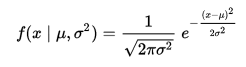
Where μ is equal to the mean of the distribution,

σ is the standard deviation,

and σ² is the variance.

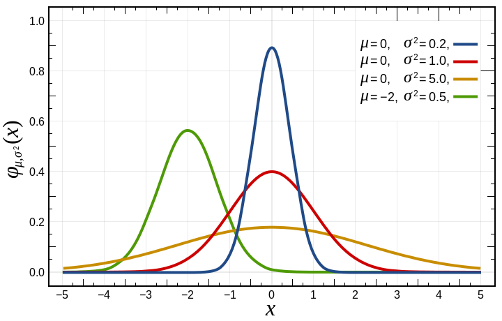
Don’t worry if the equation looks hard to understand, you can refer to the picture below for what it looks like.

Here is an example of the probability density function for a normal distribution with a few different values of μ and σ:

If you want to know how to calculate μ and σ from a data set:

Given a sample of N values (X1, X2, … XN) that has been sampled randomly from a larger set,

μ = (X1 + X2 + … + XN) / N

σ² = ((X1 - μ)² + (X2 - μ)² + … + (XN - μ)²) / (N-1)

When calculating the standard deviation σ, notice that you divide by N-1 instead of N. This adjustment is known as Bessel’s correction.

The Normal Distribution is relatively simple to work with and gives us all the information we need to draw statistical conclusions. But how do we know that our experiment will follow the Normal Distribution? We need the Central Limit Theorem for this.

Central Limit Theorem

The Central Limit Theorem is the most important theorem in experimental statistics. It states that averages of random variables with finite variance independently drawn from independent distributions become normally distributed when the number of random variables is sufficiently large. The proof is not necessary to discuss here, if you are curious here it is.

Essentially the CLT implies that if you keep pulling random samples from any sufficiently large set (finite or infinite) of independent values that has a mean μ and a variance σ², the sum of the results will converge to a normal distribution. There are plenty of caveats for that statement, but for the purposes of our experiment design we can assume it to be true.

Confidence

Finally we can talk about estimate confidence. Why was it so important to show that our data will come in with a normal distribution? Well, it’s because normally distributed data has properties we can exploit for our experiment. If we can calculate the standard deviation for our sample and collect enough samples to let the data converge to a normal distribution, we get the following effect:

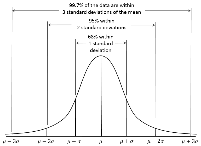
On average, we can expect 95% of our collected samples to be within 2 standard deviations of the mean, and 99.7% to be within 3. How is this useful to us? Let’s try an example.

Say we build a new feature that is supposed to improve our clickthrough rate for the checkout button (same example as in my DDDM introduction post). There are two different proposals on the table and we want to know which one is most successful, so we implement both them and release the new code experimentally to small portions of our userbase. Say we collect enough samples for the CLT to kick in and we have a good sense of what the the PDFs for these experiments look like. When we overlay them on top of each other, along with the original (control) data, it looks like this:

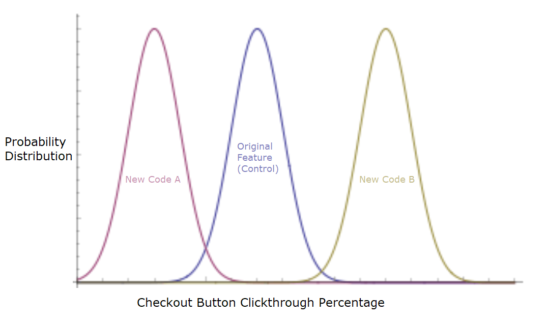
The pink curve represents proposal A, blue is the control, gold is proposal B. You can see that these curves have very little overlap: if a random customer were to encounter proposal A, we are highly confident that they are less likely to click the checkout button than if they encounter proposal B. In fact, proposal A is worse than what you had originally, and would probably result in a drop in revenue. Good thing you had the data to validate before making the mistake of checking in proposal A! In this case, proposal B would be implemented.

Experiments are not always this cut and dry. Often the PDF curves will overlap significantly, and in that case the experiment is inconclusive. But more often than not, sampling enough users will allow you to determine with a high degree of confidence which features your org should implement.

Determining Sample Size

I’ve been hand-wavy so far about there being “enough” samples to converge to a normal distribution. This is because it is dependent on some information you don’t actually know until you do the experiment! It’s a bit of a chicken and egg problem.

Appropriate sample size is determined by:

• Population size (total number of users)
• Margin of error: the margin of error you will be comfortable with. Commonly 5% is selected.
• Confidence level: How many standard deviations away from the mean indicates we are confident that our new feature is better? Commonly 95% (2 standard deviations) or 99% (3 standard deviations) is chosen.
• Standard Deviation: The standard deviation of the sample data. This has to be guessed at initially! Go for a safe value you know will not be exceeded.

Sample size is then calculated by the following:

Necessary Sample Size = (Confidence Level)² * StdDev*(1-StdDev) / (Margin of error)²

For more information, take a look at Qualtrics’ page on sample sizes.

TL;DR

In general, the appropriate process for experimental software design is:

• Determine sample size for the experiment
• Sample that number of users against a control group
• If the mean KPI we are tracking is at least 2-3 standard deviations better than the previous mean, the experiment is a success.
• In the case of success, we keep the change.
• In the case of inconclusive data, we can choose to keep our change on a case by case basis.
• In the case that the data proves the change has made a KPI worse, we roll back the change.

Test driven development is cool!